Here you can read a fragment of one of the “Seismic interpretation on 2D and 3D
” course units, that delves into reflection seismic acquisition methods
Reflection seismic acquisition methods
In this chapter we will explore the theory behind reflection seismic acquisition, some of the most important
concepts and how data acquisition is done using modern methods. We will cover 3 main topics:
– Rock properties
-Wave propagation, reflection, refraction, reflectivity, impedance
– Data acquisition ‐ onshore and offshore
Seismic interpretation on 2D and 3D
Rocks properties
Seismic waves travel through Earth’s interior as a result of earthquakes, volcanic eruptions, magma movement,
landslides or man‐made explosions.
The propagation of seismic waves will depend on the density and elasticity of the medium they travel through.
In general, the velocity of propagation increases with depth, both in the crust and in the Earth’s mantle.
Each medium (layer, geological body, etc.), depending on its composition, density, porosity, etc., will have
different physical properties, namely the velocity of wave propagation.

Types of acoustic waves
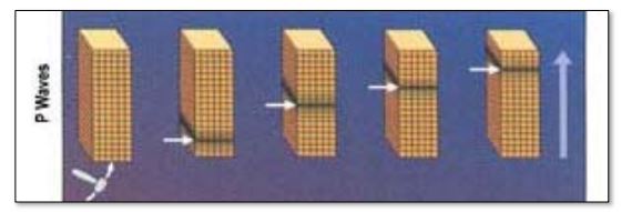
The primary waves, or P, are elastic or pressure waves, since the materials they travel through undergo
compression and rarefaction. They travel through all types of materials, solid, liquid or gaseous. Typical values for
the velocity of P waves in solid media are in the range of 5 to 8 km / s, faster than any other wave.
They are the main source of information in seismic acquisition campaigns.
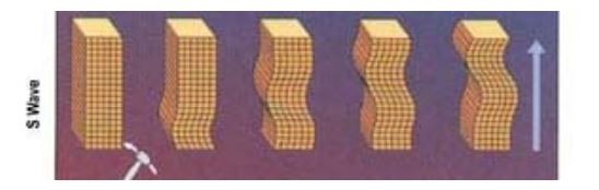
Secondary waves, or S, are shear waves, since the materials they travel through are displaced perpendicular to
the direction of propagation. They only travel through solid materials. Typical values for the velocity of S waves
are ca. 60% slower than the P waves. They are not very useful in seismic acquisition campaigns, causing some
problems in land campaigns, but they can be used for some advanced geophysical calculations.
Surface waves propagate across the Earth’s surface from the epicenter of an earthquake. There are two types of
surface waves: Rayleigh waves and Love waves. They are not generally used as acquisition data.
Properties of acoustic waves and their propagation
Acoustic waves, like other types of waves, can be characterized using several descriptive and measurable terms:
λ ‐ length is the size of a wave, the distance between two valleys or two ridges.
γ ‐ The amplitude of a wave is a measure of the magnitude of a disturbance in a medium during a wave cycle. For
example, waves on a rope have their amplitude expressed as a distance (meters).
T ‐ The period is the time of a complete cycle of an oscillation of a wave.
f ‐ Frequency is a period divided by a unit of time (example: one second), and is expressed in hertz:
f = 1 / T
v ‐ The speed of a wave is described by the following equation: v = λ.f

The velocity of wave propagation is one of the main variables for advanced geophysical interpretation.
The velocity will depend on the properties of the materials (of the rocks) it travels through as follows:
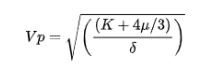
Where:
Vp P Wave velocity
K incompressibility (bulk) module
µ modulus of rigidity (for liquid materials = 0)
δ density of the material to be traversed
Wave propagation
Acoustic impedance can be defined as the set of physical properties of a medium that determine the propagation
of a wave through that medium. The impedance difference determines the amount of energy that is reflected or
refracted.

For P waves, in rock mediums, its value is determined by the density of the rock and the velocity of propagation
of P waves in that rock.

The greater the differences between the properties of the 2 layers, the greater the reflected energy ‐ and the
greater the reflectivity of the surface that divides them. In a seismic profile, the greater the reflectivity, the
greater the amplitude of that surface.
Each layer will have different density and Vp.
The contrast between layers will determine the “visibility” of the reflective surfaces, i.e. their amplitudes in a
seismic profile.
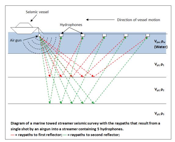
In a seismic reflection acquisition, in each layer, each point will be “analyzed” by several waves from the source‐
hydro / geophone set. In this case S1‐D1, S2‐D2, S3‐D3, etc. Each point is called Common Depth Point (CDP).
When strata are horizontal, the CDP is equivalent to a Common Mid Point (CMP).
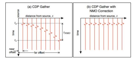
As the time that a wave takes to travel from S2 source to D2 receiver is greater than S1 to D1, the S2‐D2 trace
will be offset. The same for the S3‐D3, etc. This wave travel time between the source and the receiver (reflected
by the reflection surface) is called Two‐Way Time (TWT).

This trace offset between the several pairs of source‐receivers is called Normal Move Out and is corrected during
the first stages of processing.
The data that arrives first is called near offsets (or “nears”) and the later ones are called far offsets (or “fars”). All
are used for the final seismic product, but can be used separately for quantitative interpretation.
Seismic wave properties and propagation – some references
- Hubscher, C. and Goh, K. 2014. Reflection/Refraction Seismology Encyclopedia of Marine Geoscience. Springer
- Science
- Geophysics for Practicing Geoscientists
- SEG WIKI acquisition
- SEISMIC REFRACTION VERSUS REFLECTION