Here you can read a fragment of one of the “Applied Biostratigraphy” course units, that delves into the Numerical methods, abundance increases and maxima.
There are numerous methods to analyze biostratigraphy data numerically and/or graphically. The following chapter describes several of these methods, which will be further explored in exercises.
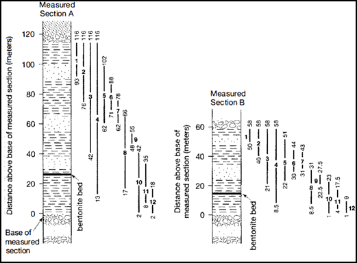
Shaw diagram
The Shaw diagram method uses the stratigraphic ranges of species in two different sections (outcrop or well). Assumes appearance and disappearance of species in the sections are synchronous (corresponding to LADs and FADs). Plots the base and top (FO and LO) of each species and any other marker (e.g. bentonite bed)
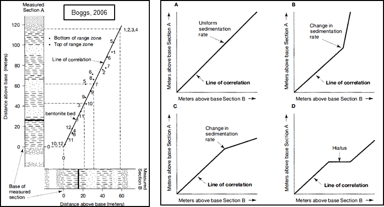
On a bivariate graph, one axis represents one section in meters and the other axis the other section, in meters. This method allows to:
- Understand changes in sedimentation rates (relative, not absolute).
- Depict hiatuses (when present in only one of the sections)
- Easy usage in short distance correlations, may prove more difficult to interpret in long distance ones.
There are some limitations of the method:
- Appearance and disappearance of species in the sections may not be synchronous, biasing the plot. This is mitigated by the use of several concurrent species (outliers can be spotted).
- Implies one section is a reference, ie, with no significant breaks.
- Requires two or more sections/wells.
Graphical correlation
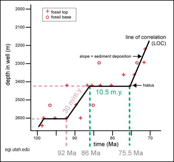
The Line of Correlation (LOC) or Sedimentation rate curves plots chronostratigraphic data (derived from species ranges or biozones) of a section, in Ma against the vertical distance of that section in meters (depth in a well or height in outcrop). It uses only one well or section per data series, but more than one well can be used in the same graphic, allowing to compare sedimentation rates in different locations. It allows to determine sedimentation rates in numerical values, depicts hiatuses and condensed sections. If well biostratigraphy is tied to seismic, ie horizons correlated with chronostratigraphic events, pseudo-wells can be made.
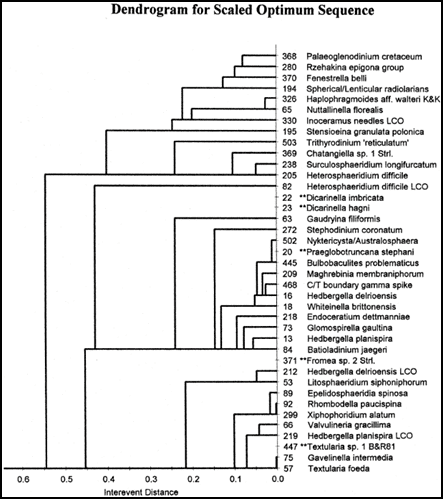
RASC correlation and CONOP9
RASC correlation is a numerical model based on the ranking of biostratigraphic events. The purpose of ranking is to create an optimum sequence of events observed in different wells or sections subject to stratigraphic inconsistencies in the direction of the arrow of time (Agterberg and Gradstein, 1999).
Constrained optimization (CONOP9) finds the best sequence of first and last appearance of fossil taxa, can handle large amounts of data from many sections, and be used to construct a composite range chart for the taxa. Both require specific software, not feasible with pencil and paper.