Here you can read a fragment of one of the “Finite element modelling in geotechnical engineering” course units.

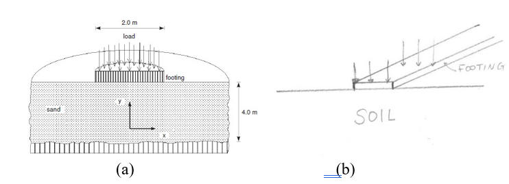
This section will show how to use a commercial software package (Plaxis 2D) to do mechanical analysis in geotechnical engineering. An example on the bearing capacity of shallow foundations will be used. The problem is 2D, plain strain for a strip footing and axisymmetric for a circular footing (Figure 3.1). Though this problem is simple, it can show the key features of mechanical analysis in geotechnical engineering, including element selection and setting up boundary and initial conditions. The basic principles to be discussed here also apply to other more complex problems.

 

 

3.1 Creating the geometry for analysis

The first step of a FEM analysis is to create the geometry. For a 2D problem, a 2D geometry is needed. In the case of circular footing, one must use half of the cross section and the left vertical side is the axis of symmetry. For the strip footing, one can use the entire cross-section. Note that half of the cross-section can also be used when the problem is symmetric about the vertical axis (e.g., the soil is composed of horizontal soil layers and there is no existing structure beside the footing).

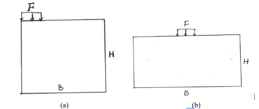
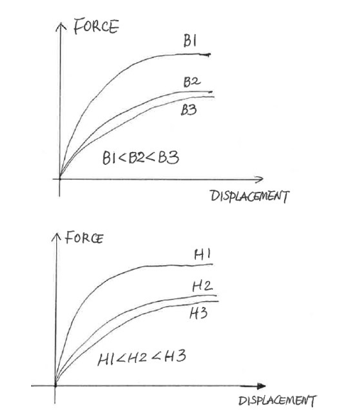
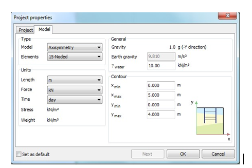
In the analysis, the force displacement relation of the footing is of concern. Therefore, we do not want the size of the geometry (or size of soil beneath the foundation) to have influence on this relation. The width of the geometry must be bigger than the width of the footing. As will be shown in the boundary conditions later, the height of the geometry should be so big that the soil does not move in either the horizontal or vertical directions at the bottom. The width of the geometry should be big enough so that there is no horizontal displacement at the right vertical side (Figure 3.2a) or both of the vertical sides (Figure 3.2b). The proper height and width of the geometry can be found by studying their effect on the force displacement relation. As the height (H1, H2, H3) and/or width (B1, B2, B3) increases, the simulated bearing capacity (the maximum value of the force) will decrease (Figure 3.3). The reason is that smaller height and width will give more confinement to the soil and make the soil stronger. However, when the width and height and width is big enough, further change in then will have little effect on the bearing capacity. Such critical width and height should be used in the analysis. For the case shown in Figure 3.3, B2 and H2 are essentially big enough for the analysis. In Plaxis 2D, the contour option is used to set the size of the geometry (Figure 3.4).

 

 

 

3.2 Selecting the element type

The element is crucial for the FEM analysis. First, one needs to decide whether the problem is 2D or 3D. In geotechnical engineering, the 2D analysis is more widely used, even for some 3D problems. This is because the 3D analysis is more computationally expensive and the geometry is harder to create. Indeed, the 2D analysis does offer reasonable solutions. For the 2D analysis, one should choose either plain strain or axisymmetric element according to the problem features (see the Type option in Figure 3.4). In each FEM software package, there are several options for the geometry and node numbers of elements. Generally, elements with more nodes give more accurate results. But the computational time will be longer if there are more nodes in the problem. In Plaxis 2D, the only element geometry available is triangle. One can select 6-noded or 15-noded elements (see the Type option in Figure 3.4).

3.3 Selecting the element size

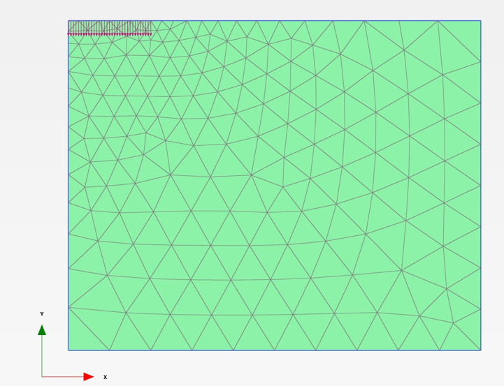
In FEM analysis, a problem is discretized into small meshes (Figure 3.5). The mesh size has significant influence on the solutions. Generally, smaller mesh size (smaller element) gives more accurate solutions, as the simulated deformation field is more accurate. When the problem shown in Figure 3.5 is simulated using 2 or 3 elements (very big mesh size), the soil will behave more like a rigid body, which indicates the solution will be far from being accurate. Therefore, the mesh size should be small enough. For the shallow foundation problem, one can find out the proper mesh size by investigating the effect of mesh size on the force and displacement relation of the footing. Finer mesh will make the soil more flexible and the simulated bearing capacity smaller (Figure 3.6). When the mesh size is small enough, further decrease in mesh size will not affect the solution.

 

 

3.4 Setting up the boundary conditions

There are different types of boundary conditions for geotechnical problems. Here are some examples:

Mechanical analysis (force displacement relation is of concern):

• Deformation boundary conditions
• Stress or force boundary conditions

Consolidation analysis (force displacement relation and change in excess pore pressure is of concern):

• Deformation and stress/force boundary conditions
• Boundary conditions for water flow (called water conditions in Plaxis) Seepage analysis (water flow is of concern):
• Permeable or impermeable boundary (called water conditions in Plaxis)
• Flow velocity at the boundaries

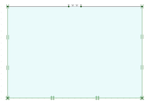
Note the boundary conditions may change at different analysis stages. For the shallow foundation problem here, the deformation boundary conditions need to be specified for the bottom and two vertical sides. At the bottom, the soil neither move horizontally nor vertically. At the two vertical sides, only vertical movement is possible. This kind of boundary condition is called ‘default fixities’ in Plaxis (Figure 3.7). Indeed, this boundary condition can be used a lot of mechanical problems for soils.

 

3.5 Setting up the initial conditions

Initial conditions are very important for FEM analysis involving soils. For example, the initial stress state will affect the simulated bearing capacity of a footing when the soil is modelled using the Mohr-Coulomb failure criterion. For example, it the initial effective stress state is very close to the Mohr-Coulomb failure curve, the predicted bearing capacity will be very low. Generally, there are two types of initial conditions:  • Water condition (or initial pore pressure state)

• Initial effective stress state.

In Plaxis, the water condition can be set by specifying the water head in geometry creation. The software will calculate the initial pore pressure distribution automatically. The water density can be changed in the project definition (𝛾_{𝑤𝑎𝑡𝑒𝑟} in Figure 2.18). In other software packages, you may need to give initial pore pressure distribution directly.

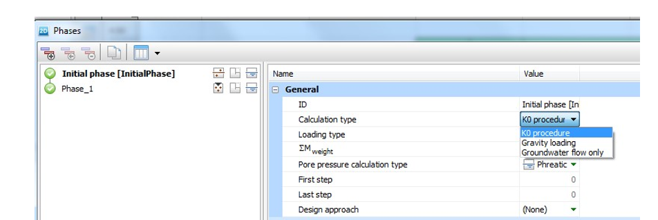
We will use Plaxis to show how to generate the initial effective stress state. First, you need to select the method for generating the initial effective stress state in the initial phase of the analysis (Figure 3.8):

• 𝐾₀ procedure
• Gravity loading procedure

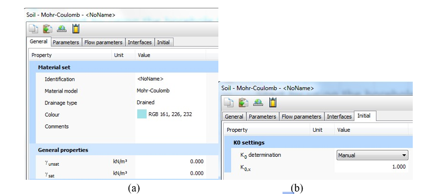
In order to generate the initial effective stress state, the following parameters needed to be given (Figure 3.9)

• Saturated unit weight of soil 𝛾_𝑠𝑎𝑡
• Unsaturated unit weight of soil 𝛾_{𝑢𝑛𝑠𝑎𝑡}
• Later earth pressure coefficient 𝐾_0𝑥

The initial effective stress state is calculated by two steps

• Step 1: Calculate the vertical effective stress σ’_y (see Figure 2.2 for the coordination system definition)
• Step 2: Calculate the horizontal effective stress σ’_x (=σ’_z)

These two steps will be discussed for the 𝐾₀ procedure and gravity loading procedure, respectively.

 

 

 

 

The 𝐾₀ procedure:

Step 1:

σ’_y = 𝛾’h

Step 2:

σ’ _x = K h_0x 𝛾’h and σ’ _z = K h_0x 𝛾’h

where

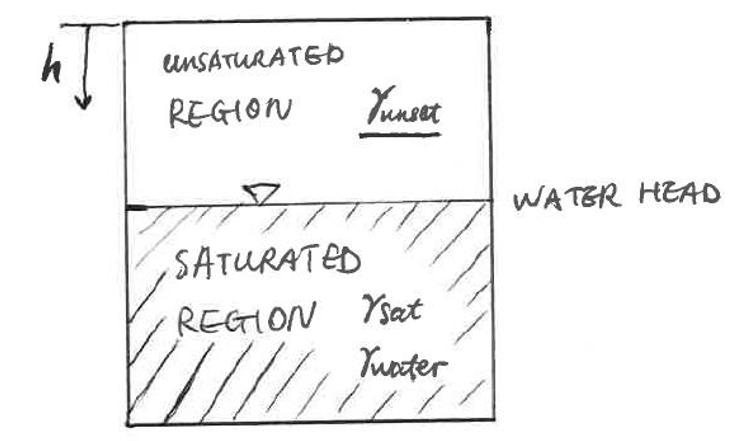
𝛾’ = 𝛾’ _unsat in the unsaturated region

𝛾’ = 𝛾’ _sat − 𝛾 _water in the unsaturated region

h : depth of the soil from the surface (Figure3.10)

 

For this procedure, the most important parameter is K_0x . It can be given by manual input or automatic calculation by Plaxis (Figure 3.9b). The automatic calculation by Plaxis gives K_0x using the Jack’s equation

K_0x = −1 sin𝜑’

where 𝜑’ is the friction angle of soils. Note that the lateral earth pressure coefficient is dependent on overconsolidation ratio (OCR) of soils. Mayne and Kulhawy proposed the following equation for overconsolidated soils and it is now widely used

K_0x = (1−sin 𝜑’)OCR^{sin 𝜑’}

Therefore, K_0x should be specified manually when the soil is not normally consolidated (Figure 3.9b). Indeed, the K_0x has significant effect on the solution when the Mohr-Coulomb failure criterion is used in the mechanical analysis.

 

Gravity loading procedure

The 𝐾₀ procedure is only valid when for some special cases (e.g., horizontal soil layers, horizontal water head and no other structures such as piles). For instance, it cannot be used for the cases shown in Figure 3.11. This is because σ’_y ≠ 𝛾’h under these conditions. The gravity loading procedure must be used.

 

For this procedure, the initial effective stress state is calculated as below (please refer to Figure 2.2 for the coordination system definition): Step 1:

σ’_y = Actual soil weight (water pressure is excluded in the saturated region)

σ’x = K0x σ’_y and σ’z = K0x σ’_y

where

K0x =  ν’ / 1- ν’

where ν’ is the Poisson’s ratio of the soil. The K₀ is derived by assuming that the initial state is one-dimensional consolidation (zero strain in the horizontal direction and

σ’z = σ’x) and the soil is behaving elastically. According to the Hook’s law, one can get the following equation for one-dimensional consolidation

and therefore,

where      is the elastic strain in the x-direction.

3.5 Specifying material properties

The material properties are the most important for the FEM analysis. If the material properties (especially those for soils) are not properly specified, the solutions can be totally wrong. This course will focus on the material properties for soils. To specify the properties for soils, one needs to select a proper constitutive model and then give the proper model parameters. The following section will focus on this.

3.6 Errors in FEM analysis

The FEM simulations give approximate solutions for real boundary value problems. Therefore, there are always errors in the solutions. You can make the errors as small as possible but not vanish. There are many sources of errors. Some of them will be discussed below:

• A real boundary value problem is idealized to be an assembly of elements. Such discretization assumes that there are limited degrees of freedom for the problem.

However, a real boundary value problem has infinite numbers of degrees of freedom. This approximation also makes the FEM solutions mesh-dependent.

• Rigorously speaking, there are no 2D problems. Some problems are approximately plane strain or axisymmetric.
• Constitutive models are indispensable for FEM analysis. However, constitutive models can only offer simplified description of soil behaviour. More advanced models can give predictions closer to the real soil behaviour, and thus, can help to reduce the error. But there is always difference between the model prediction and real soil response. This is one of the major sources of errors in FEM analysis in geotechnical engineering.
• There are also errors associated with integration of the constitutive models in the FEM code and solving the global force-displacement equations.

Therefore, when the FEM solutions are used or interpreted, these potential errors should be properly considered. One should also use the common sense to judge the solutions (Is the bearing capacity unreasonably high or low? Is the failure or deformation mode reasonable?).