Here you can read a fragment of one of the “Geostatistics for exploration and mining” course units, that delves into the Numerical methods of estimation.
Methods of estimation
Several methods of point and block estimation exist, from the simplest to the most complicated, and they all have their champions. Here we will briefly discuss a few of them, such as linear interpolation, polygon estimation, estimation by inverse distance, estimation by fixed radius local averaging, and natural neighbors estimation.
Estimation by linear interpolation
We already discussed this estimation method when talking about spatial data representation in the previous unit (section 5.2): indeed in order to construct our isopleths (or isoconcentration) lines, we have to somehow estimate the values at any point in the study area. Linear interpolation, as noted in Unit 5, relies on the assumption that the concentrations between two points of known values follow a linear relationship as a function of the distance between the points. Thus, knowing the distance between the two points and the values at the two locations, we can easily calculate the concentration for any point in between. This is a classic and mathematically straightforward method that has been in use for quite some time; however, it is significantly hampered by the fact that in geology there is rarely linear relationship between concentrations and distance.
Estimation by inverse distance
This method uses the distance between the point estimated and the available data points as a weighing factor: the farther the known point, the lower its participation in the estimation of the unknown point is. This method relies on the idea that the closer two points are to each other, the closer their concentrations will be to each other; the assumption is that at zero distance the concentrations will be the same, and at large distance they will be very different, to the point of being independent. The difficulty with this method is deciding how many points to use: the minimum is just the nearest three and the maximum is all points available. We do not have any independent factor or consideration allowing us to decide how many points to use; thus, geochemists are reduced to arbitrarily deciding on a number of known points to use or on the distance within which points are taken into consideration. Another difficulty is deciding what shape the distance vs. weight relationship we should use: linear, or quadratic, or polynomial? These are all common weighing models in the inverse distance estimation method, but how do we select the one that is most appropriate for our situation?
Estimation by polygons
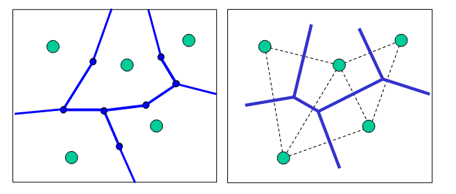
The idea here is that we design specific polygons based on the position of the points of known value and then assign the value of the point at the centre of the polygon to the whole polygon. There are two main methods of designing polygons (Thiessen and Delaunay polygons: Fig. 6.2), but the idea is exactly the same.
Estimation by fixed radius local averaging
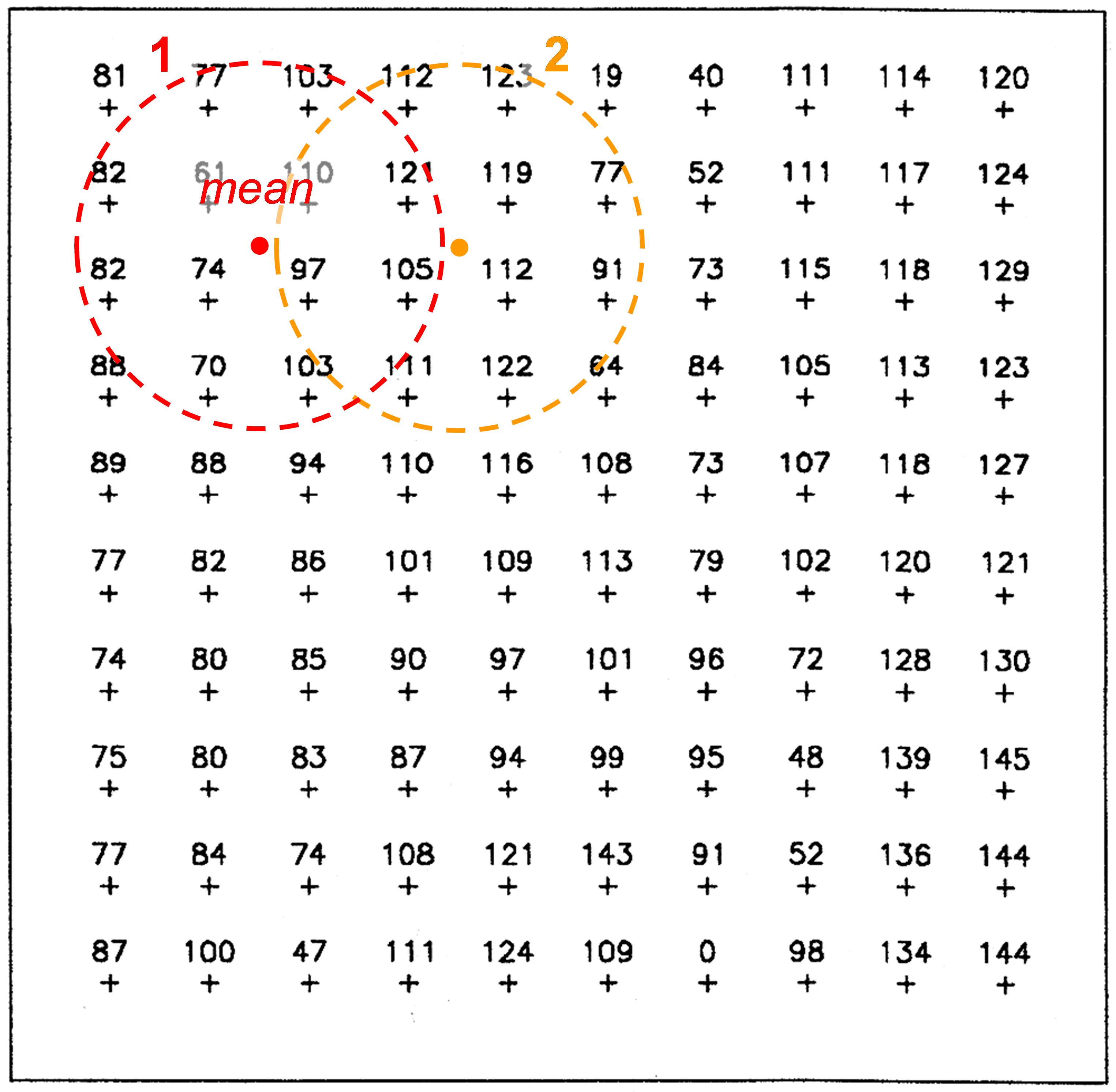
Again, this is a method that we discussed in Unit 5. The idea is that we arbitrarily define an area, let’s say a circle, and average all the known values that fall within this area as we move it around on the study area; we assign the average value to the centre of this area (Fig. 5.10, 6.3).
Natural neighbour estimation
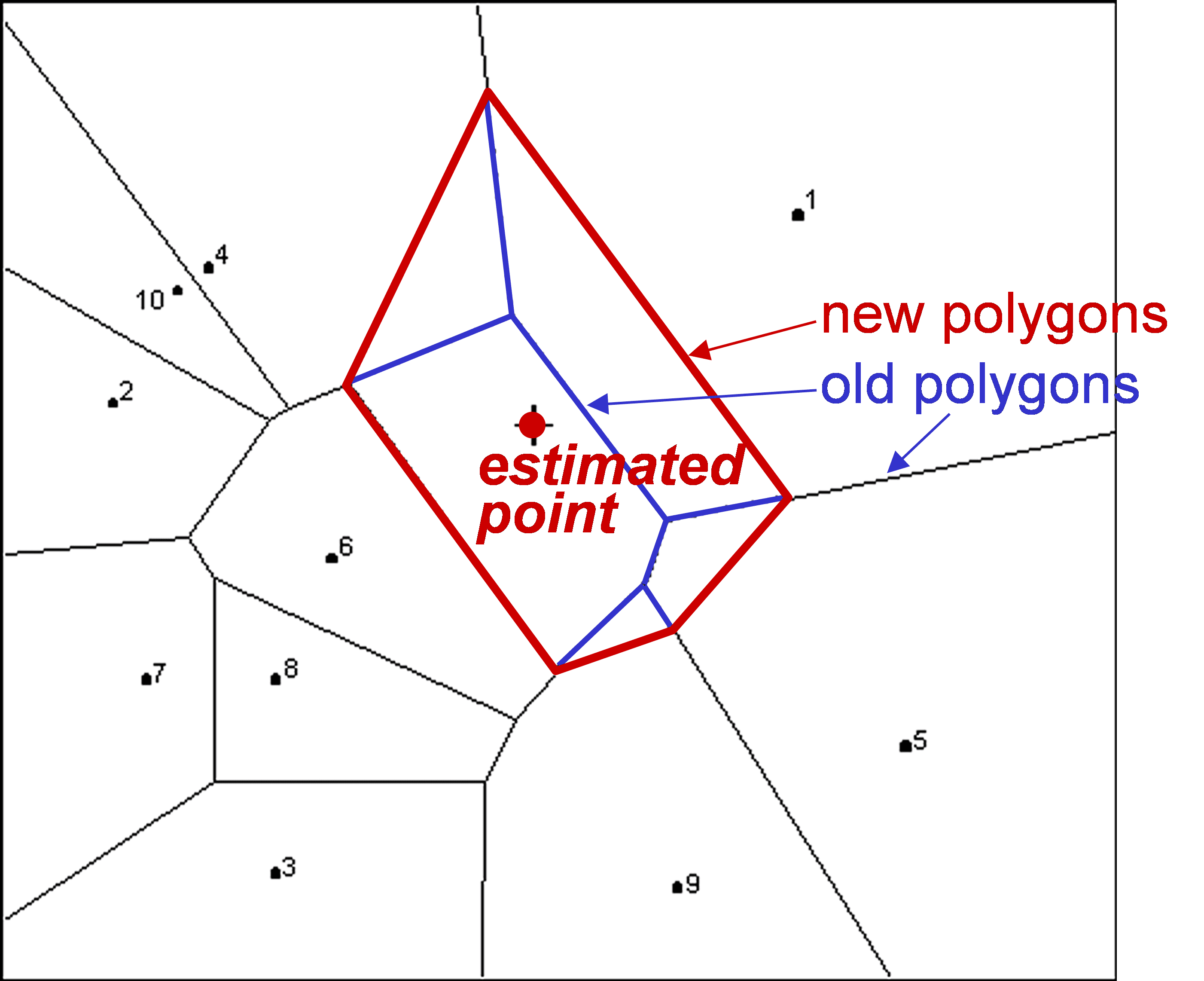
Natural neighbour is a somewhat complicated method, based on the intersection of polygons drawn with or without the estimated point. Firstly, Thiessen or Delauney polygons are drawn, with one data point per polygon; each of these polygons takes the known value. Then we draw new polygons, based on the point we want to estimate. The “old” polygons and the “new” polygons overlap to a certain degree: the new polygon is made of bits of the old polygons with different sizes (Fig. 6.4). The concentration for the estimated point is calculated using the known values in the old polygons (only those participating in the new one), and on their proportion in the new polygon: the larger their proportion in the new polygon, the more weight is given to that value. Yes, the method is clunky and its logic not clearly apparent, yet it has its valiant and vigorous defenders.
Strengths and weaknesses of these estimation methods
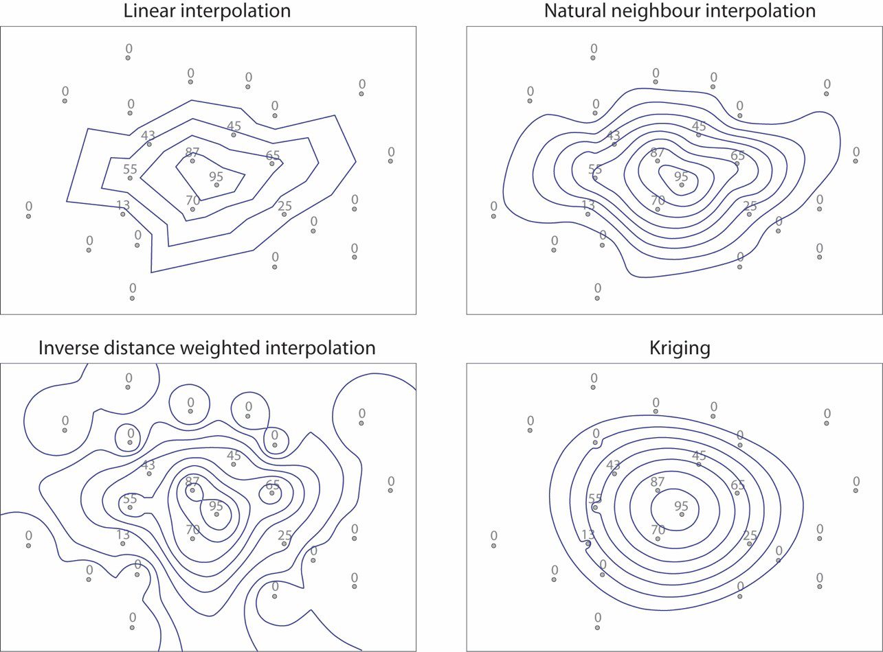
When we consider these five methods of estimating values anywhere in the study area, we notice certain commonalities: they all rely on some shared basic assumptions. The major among these is that there is no concentration difference between samples collected immediately next to each other; in other words we assume that there is no zero-distance variability or uncertainty. The second commonality is that no pre-existent (background) geological variability is taken into account, and more specifically, it is assumed that there is no preferential background geochemical heterogeneity or orientation in the study area. Finally, we always use some sort of weighing: distance in linear and inverse-distance interpolations, and polygon overlap proportion in the natural neighbour method. This is, of course, a useful and logical approach; the only question is what reasoning is followed in assigning the weights and in deciding which the weighing factor will be. The methods discussed here use purely geometrical weighing factors and arbitrarily assigned assumptions (e.g., linear lateral variability) and limitations (e.g., number of points to consider), without any attempt to provide some sound reason for these assumptions and limitations. This alone should disqualify these methods, also considering the extreme variability of results (Figure. 6.5): indeed, which one should the impartial practitioner select and why? In other words, there would be some specific reasons behind following any of these methods, and these should, ideally, follow geological reality.